Quantile Regression in the Presence of Monotone Missingness with Sensitivity Analysis

2014 ENAR Presentation

Minzhao Liu, Department of Statistics, The University of Florida
Mike Daniels, Department of Integrative Biology, The University of Texas at Austin

Quantile Regression

engel

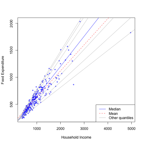
  • Engel data on food expenditure vs household income for a sample of 235 19th century working class Belgian households.
  • More information from quantile regression
    • Slope change
    • Skewness
  • Less sensitive to heterogeneity and outliers

Monotone Missingness

A missing data pattern is monotone if, for each individual, there exists a measurement occasion \(j\) such that \(R_1 = ··· = R_{j−1} = 1\) and \(R_j = R_{j+1} = · · · = R_J = 0\); that is, all responses are observed through time \(j − 1\), and no responses are observed thereafter. \(S\) is called follow-up time.

Subject T1 T2 T3 T4 S
Subject 1 \(Y_{11}\) \(Y_{12}\) 2
Subject 2 \(Y_{21}\) \(Y_{22}\) \(Y_{23}\) \(Y_{24}\) 4
  • Assumption: \(Y_{i1}\) is always observed.
  • Interested: \(\tau\)-th marginal quantile regression coefficients \(\mathbf \gamma_j = (\gamma_{j1}, \gamma_{j2}, \ldots, \gamma_{jp})^T\), \[ Pr (Y_{ij} \leq \mathbf x_i^{T} \mathbf \gamma_j ) = \tau, \mbox{ for } j = 1, \ldots, J, \] \[ p_k(Y) = p(Y | S = k), \quad p_{\geq k} (Y) = p(Y | S \geq k) \]

Pattern Mixture Model

  • Mixture models factor the joint distribution of response and missingness as \[ p (\mathbf Y, \mathbf S |\mathbf x, \mathbf \omega) = p (\mathbf Y|\mathbf S, \mathbf x, \mathbf \omega) p (\mathbf S | \mathbf x, \mathbf \omega). \]
  • The full-data response distribution is given by \[ p (\mathbf Y | \mathbf x, \mathbf \omega) = \sum_{S \in \mathcal{S}} p(\mathbf Y| \mathbf S, \mathbf x, \mathbf \theta) p (\mathbf S | \mathbf x, \mathbf \phi), \] where \(\mathcal{S}\) is the sample space for follow-upch time \(S\) and the parameter vector \(\mathbf \omega\) is partitioned as \((\mathbf \theta, \mathbf \phi)\).
  • The conditional distribution of response within patterns can be decomposed as \[ P (Y_{obs}, Y_{mis} | \mathbf S, \mathbf \theta) = P (Y_{mis}|Y_{obs}, \mathbf S, \mathbf \theta_E) Pr (Y_{obs} | \mathbf S, \mathbf \theta_{y, O}), \]
  • \(\mathbf \theta_E\): extrapolation distribution
  • \(\mathbf \theta_{y, O}\) : distribution of observed responses

Model Settings

  • Multivariate normal distributions within each pattern \[ \begin{align} Y_{i1}|S_i = k & \sim N (\Delta_{i1} + \mathbf \beta_1^{(k)}, \sigma_1^{(k)} ), k = 1, \ldots, J,\\ Y_{ij}|\mathbf Y_{ij^{-}}, S_i = k & \sim \begin{cases} \textrm{N} \big (\Delta_{ij} + \mathbf y_{ij^{-}}^T \mathbf \beta_{Y,j-1}, \sigma_j \big), & k \geq j ; \\ \textrm{N} \big ( \chi(\mathbf x_{i}, \mathbf Y_{ij^{-}}), \sigma_j \big), & k < j ; \\ \end{cases}, \mbox{ for } 2 \leq j \leq J, \\ S_{i} = k|\: \mathbf x_{i} & \sim \textrm{Multinomial}(1, \mathbf \phi). \end{align} \]
  • The marginal quantile regression models: \[ Pr (Y_{ij} \leq \mathbf x_{i}^T \mathbf \gamma_j ) = \tau, \]
  • \(\chi(\mathbf x_{i}, \mathbf y_{ij^{-}})\) is the mean of the unobserved data distribution and allows sensitivity analysis by varying assumptions on \(\chi\); for computational reasons, we assume that \(\chi\) is linear in \(y_{ij^{-}}\).
  • Here we specify \[ \chi(\mathbf x_{i}, \mathbf y_{ij^{-}}) = \Delta_{ij} + \mathbf y_{ij^{-}}^T \mathbf \beta_{y,j-1} + h_{0}^{(k)}. \]

\(\Delta\)

\(\Delta_{ij}\) are subject/time specific intercepts determined by the parameters in the model and are determined by the marginal quantile regressions, \[ \tau = Pr (Y_{ij} \leq \mathbf x_{i}^T \mathbf \gamma_j ) = \sum_{k=1}^J \phi_kPr_k (Y_{ij} \leq \mathbf x_{i}^T \mathbf \gamma_j ) \mbox{ for } j = 1, \] and \[ \begin{align} \tau &= Pr (Y_{ij} \leq \mathbf x_{i}^{T} \mathbf \gamma_j ) = \sum_{k=1}^J \phi_kPr_k (Y_{ij} \leq \mathbf x_{i}^{T} \mathbf \gamma_j ) \\ & = \sum_{k=1}^J \phi_k \int\cdots \int Pr_k (Y_{ij} \leq \mathbf x_{i}^{T} \mathbf \gamma_j | \mathbf y_{ij^{-}} ) p_k (y_{i(j-1)}| \mathbf y_{i(j-1)^{-}}) \nonumber \\ & \quad \cdots p_k (y_{i2}| y_{i1}) p_k(y_{i1}) dy_{i(j-1)}\cdots dy_{i1}. \mbox{ for } j = 2, \ldots, J .\nonumber \end{align} \]

Intuition

  • Embed the marginal quantile regressions directly in the model through constraints in the likelihood of pattern mixture models
  • The mixture model allows the marginal quantile regression coefficients to differ by quantiles. Otherwise, the quantile lines would be parallel to each other.
  • The mixture model also allows sensitivity analysis.

Missing Data Mechanism and Sensitivity Analysis

  • Mixture models are not identified due to insufficient information provided by observed data.
  • Specific forms of missingness are needed to induce constraints to identify the distributions for incomplete patterns, in particular, the extrapolation distribution
  • In mixture models , MAR holds (Molenberghs et al. 1998; Wang & Daniels, 2011) if and only if, for each \(j \geq 2\) and \(k < j\): \[ p_k(y_j|y_1, \ldots, y_{j-1}) = p_{\geq j}(y_j|y_1, \ldots, y_{j-1}). \]

Sensitivity Analysis

\[ Y_{ij}|\mathbf Y_{ij^{-}}, S_i = k \sim \begin{cases} \textrm{N} \big (\Delta_{ij} + \mathbf y_{ij^{-}}^T \mathbf \beta_{Y,j-1}, \sigma_j \big), & k \geq j ; \\ \textrm{N} \big (\Delta_{ij} + \mathbf y_{ij^{-}}^T \mathbf \beta_{y,j-1} + h_{0}^{(k)}, \sigma_j \big), & k < j ; \\ \end{cases}, \mbox{ for } 2 \leq j \leq J, \]

  • When \(2 \leq j \leq J\) and \(k < j\), \(Y_j\) is not observed, thus \(h_0^{(k)}\) can not be identified from the observed data.
  • \(\mathbf \xi_s = (h_0^{(k)})\) is a set of sensitivity parameters (Daniels & Hogan 2008), where \(k =1, ..., J-1\).
  • \(\mathbf \xi_s = \mathbf \xi_{s0} = \mathbf 0\), MAR holds.
  • \(\mathbf \xi_s\) is fixed at \(\mathbf \xi_s \neq \mathbf \xi_{s0}\), MNAR.
  • We can vary \(\mathbf \xi_s\) around \(\mathbf 0\) to examine the impact of different MNAR mechanisms.

MLE

The observed data likelihood for an individual \(i\) with follow-up time \(S_i = k\) is \[ \begin{align} L_i(\mathbf \xi| \mathbf y_i, S_{i} = k) & = \phi_kp_k (y_k | y_1, \ldots, y_{k-1}) p_k (y_{k-1}|y_1, \ldots, y_{k-2}) \cdots p_{k} (y_1), \\ & = \phi_k p_{\geq k} (y_k | y_1, \ldots, y_{k-1}) p_{\geq k-1} (y_{k-1}|y_1, \ldots, y_{k-2}) \cdots p_{k} (y_1), \nonumber \end{align} \]

  • To facilitate computation of the \(\Delta\)'s and the likelihood, we propose a tricky way to obtain analytic forms for the required integrals.
  • Use the bootstrap to construct confidence interval and make inferences.

Real Data Analysis: Tours

Subject 6 Months 18 Months Age Race Baseline
Subject 1 \(Y_{11}\) \(Y_{12}\) \(x_{11}\) \(x_{12}\) \(Y_{10}\)
Subject 2 \(Y_{21}\) \(Y_{22}\) \(x_{21}\) \(x_{22}\) \(Y_{20}\)
  • Weights were recorded at baseline (\(Y_0\)), 6 months (\(Y_1\)) and 18 months (\(Y_2\)).
  • We are interested in how the distributions of weights at six months and eighteen months change with covariates.
  • The regressors of interest include AGE, RACE (black and white) and weight at baseline (\(Y_0\)).
  • Weights at the six months (\(Y_1\)) were always observed and 13 out of 224 observations (6%) were missing at 18 months (\(Y_2\)).
  • The AGE covariate was scaled to 0 to 5 with every increment representing 5 years.
  • We fitted regression models for bivariate responses \(\mathbf Y_i = (Y_{i1}, Y_{i2})\) for quantiles (10%, 30%, 50%, 70%, 90%).
  • We ran 1000 bootstrap samples to obtain 95% confidence intervals.

Results

engel

  • For weights of participants at six months, weights of whites are generally 4kg lower than those of blacks for all quantiles significantly.
  • Weights of participants are not affected by age significantly.
  • Coefficients of baseline weight show a strong relationship with weights after 6 months.
  • For weights at 18 months after baseline, we have similar results.
  • However, whites do not weigh significantly less than blacks at 18 months unlike at 6 months.

Sensitivity Analysis

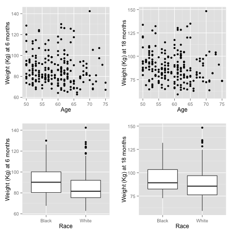
We also did a sensitivity analysis based on an assumption of MNAR.

  • Based on previous studies of pattern of weight regain after lifestyle treatment (Wadden et al. 2001; Perri et al. 2008) we assume that \[ E(Y_2 - Y_1| R=0) = 3.6 \mbox{kg}, \] which corresponds to 0.3kg regain per month after finishing the initial 6-month program.
  • Specify \(\chi(\mathbf x_{i}, Y_{i1})\) as \[ \chi(\mathbf x_{i}, y_{i1}) = 3.6 + y_{i1}, \]

  • There are no large differences for estimates for \(Y_2\) under MNAR vs MAR.

  • This is partly due to the low proportion of missing data in this study.

Summary

  • Developed a marginal quantile regression model for data with monotone missingness.
  • Used a pattern mixture model to jointly model the full data response and missingness.
  • Estimate marginal quantile regression coefficients instead of conditional on random effects.
  • Allows for sensitivity analysis which is essential for the analysis of missing data (NAS 2010).
  • Allows the missingness to be non-ignorable.
  • Recursive integration simplifies computation and can be implemented in high dimensions.

Future Work

  • Simulation results showed that the mis-specification of the error term did have an impact on the extreme quantile regression inferences.
  • Working on replacing it with a non-parametric model, for example, a Dirichlet process with mixture of normals.